zkML: Tradeoffs in accuracy vs. proving cost
In the land of (zk)SNARKS, building the most accurate machine learning model is often at odds with the costs of proving and verifying model inference.
To demonstrate the tradeoffs between model accuracy and SNARK costs, we’ve implemented a proof-of-concept using the EZKL zkML framework. Our goal is to highlight how small increases in accuracy might lead to significant computational expenses, encouraging thoughtful consideration of these tradeoffs when building models that need verifiability. This post provides a detailed explanation of the process, including data preprocessing, model training, and proof generation.
As proof-of-concept, we’ve chosen a Token Trend Forecasting task. This task involves binary classification, aiming to predict whether a token’s price will rise or fall in the future. zkML is particularly relevant for blockchain applications, and besides price prediction, it can also be useful for other critical tasks in the blockchain space, such as forecasting market volatility and assessing investment risk, as well as many non-financial applications.
zkML Frameworks
We are interested in a generic framework that can be used to prove the inference of any ML model. A common format for representing ML models is ONNX, which is supported by most popular ML frameworks such as PyTorch or TensorFlow. It allows for interoperability between different ML frameworks and tools.
At the time of writing, we found two zkML frameworks that can convert models saved as ONNX files into SNARK circuits. These are GIZA and EZKL.
EZKL is a Halo2-based zkML framework developed by zkonduit. It is designed to work with any computational-graph-based ML model, which makes it flexible enough to support most of the popular ML frameworks (e.g., TensorFlow, PyTorch, etc.). It provides a simple Python API that allows users to easily prove inference results, abstracting away the complexities of the proof system.
GIZA relies on Cairo, a general-purpose language for provable computation, as its zkSTARK backend. It is Rust-based and provides a more low-level API compared to EZKL. The entire Giza stack is designed around the Cairo language. It offers several tools and libraries to help users build models and prove their results. Among them are Orion, which allows users to transpile their Python models to Cairo, and Giza Hub, which offers a collection of models and use cases.
We decided to build our PoC using EZKL, as at the time of writing, Giza was experiencing some issues when proving inference of their deployed models (e.g., this issue). However, we believe that the methodology described here could easily be applied to models built with Giza or other zkML frameworks.
EZKL Workflow
This section provides a high-level overview of the workflow to prove the inference of a trained model using EZKL. Let’s assume that we have just trained a simple perceptron on a MNIST classification task model using PyTorch:
import torch
import torch.nn as nn
from torch.utils.data import DataLoader
import torchvision

# MNIST dataset
train, test = (torchvision.datasets.MNIST(
    './data',
    train=is_train,
    transform=torchvision.transforms.Compose([
        torchvision.transforms.ToTensor(),
        torchvision.transforms.Normalize((0.1307,), (0.3081,)),
        torchvision.transforms.Lambda(lambda x: x.view(-1))
    ])
) for is_train in [True, False])

input_size, output_size = 28 * 28, 10

# Define the model
perceptron = nn.Sequential(
    nn.Linear(input_size, output_size),
)

# Create a dataset and data loader
train_loader, test_loader = (DataLoader(
    dataset,
    batch_size=32,
    shuffle=True
) for dataset in [train, test])

# Define the loss function and optimizer
criterion = nn.CrossEntropyLoss()
optimizer = torch.optim.Adam(perceptron.parameters(), lr=0.01)

# Train the model
perceptron.train()
for data, label in train_loader:
    output = perceptron(data)
    loss = criterion(output, label)
    optimizer.zero_grad()
    loss.backward()
    optimizer.step()
The steps to bring prove and verify inference of the model using EZKL are as follows:
ONNX Conversion: This conversion process is streamlined by specific functions available in most machine learning frameworks. For example, PyTorch models can be converted using the
torch.onnx.exportfunction. In other instances, conversion tools are found in external libraries. For instance, thetf2onnxpackage facilitates the conversion of TensorFlow models to ONNX format.In cases where a direct conversion tool is not available, a workaround involves casting the model to a different framework before conversion. For instance, some Sklearn models such as decision trees must be first converted to PyTorch using
hummingbird.ml. We won’t cover the process in this article but more information can be found in the following EZKL’s notebook.Before converting a model to the ONNX format, we must specify the model’s input structure. This means specifying the shape and type of the input expected by the model. To do this, we typically use a dummy input tensor, which can be randomly generated or taken from one of the datasets. In this example, we use the first input from the test dataset:
import json # Choose any valid input tensor (1st input of the test dataset) input_sample = next(iter(test_loader))[0][0].unsqueeze(0) torch.onnx.export( perceptron, input_sample, "perceptron.onnx", input_names = ['input'], # Input and output labels to appear in the ONNX graph output_names = ['output'], dynamic_axes={ 'input' : {0 : 'batch_size'}, # Variable length axes 'output' : {0 : 'batch_size'} } )Setup: EZKL has several setup functions in their exposed API, namely
gen_settings,calibrate_settings,compile_circuit,get_srs,setup, andgen_witness. We have grouped them together in two bullet points to describe the high level process:Calibration functions: includes
gen_settingsandcalibrate_settings. Thegen_settingsfunction generates a generic settings file that contains the metadata required for proving the inference of the model. The subsequent call tocalibrate_settingswill adjust the file to the specific model and input data. The internal calibration process is very complex and involves several steps, such as determining the number of constraints, the number of variables, scales, lookup ranges, etc. EZKL abstracts this complexity away from the user, making it easier to use. There is, however, a tradeoff between the calibration process and the proving cost. In particular, there is a valuelogrowsthat represents the size of the polynomials committed to using KZG. That value can oscillate one or two units up or down for models with the same architecture. Of course, this affects the accuracy of the quantized model EZKL proves. Furthermore, the proof generation time is exponentially proportional to the value oflogrows.PCS Setup: involves
compile_circuit,get_srs,gen_witness, andsetup. Thecompile_circuitfunction converts the ONNX model to an arithmetic circuit.get_srsretrieves the structured reference string, which is required to compute the prover and verifier keys. Thegen_witnessmethod uses the input data and the compiled model to generate a witness for the proof. Finally, thesetupfunction generates the verification and proving keys required for the proof generation.
More information can be found in the EZKL documentation. For our purposes, we will use the following code snippet to run the setup process:
import ezkl
import json

def create_file(filename: str) -> str:
    open(filename, 'w').close()
    return filename

# We have to create empty files manually before running the setup
INPUT = create_file("input_data.json")
SETTINGS = create_file("settings.json")
CALIBRATION = create_file("calibration.json")
WITNESS = create_file("witness.json")
COMPILED_MODEL = create_file("compiled_model.json")
VK = create_file("vk.json")
PK = create_file("pk.json")
PROOF = create_file("proof.pf")

def setup(model, onnx_file, input_sample):

    # Save the input data to a file in the expected format
    input_data = {
        'input_shapes': list(input_sample.shape),
        'input_data': input_sample.detach().numpy().tolist(),
        "output_data": model(input_sample).detach().numpy().tolist()
    }

    json.dump(
        input_data,
        open(INPUT, 'w')
    )

    # Run each setup function and verify that it succeeded
    assert ezkl.gen_settings(
        onnx_file,
        SETTINGS
    )

    json.dump(
        input_data,
        open(CALIBRATION, 'w')
    )

    assert ezkl.calibrate_settings(
        INPUT,
        onnx_file,
        SETTINGS,
        "resources"
    )

    assert ezkl.compile_circuit(
        onnx_file,
        COMPILED_MODEL,
        SETTINGS
    )

    assert ezkl.get_srs(
        SETTINGS
    )

    ezkl.gen_witness(
        "input_data.json",
        COMPILED_MODEL,
        WITNESS
    )

    assert ezkl.setup(
        COMPILED_MODEL,
        VK,
        PK
    )

setup(perceptron, "perceptron.onnx", input_sample)
Proof generation and verification: We can easily generate the proof using the
provefunction. This function takes the arithmetization of the model, the witness, the public key, and the (empty) proof file as inputs and writes the proof into said file.verifythen is used to verify that proof:import pprint proof = ezkl.prove( WITNESS, COMPILED_MODEL, PK, PROOF, "single", ) pprint.pprint(proof) >> { 'instances': [ ['df...00', 'd8...30', ..., '13...30'] ], 'proof': '0x1d....1f', 'transcript_type': 'EVM' } ezkl.verify( PROOF, SETTINGS, VK ) >> True
Token Trend Forecasting
As mentioned earlier, our chosen proof-of-concept task of Token Trend Forecasting involves binary classification, aiming to predict whether a token’s price will rise or fall in the future. Since zkML is particularly relevant for blockchain applications, we consider this task to be a good example of how zkML can be adopted in the future financial industry.
We have adapted code from the following GIZA’s example. Our modifications include changes to make the code more readable and to better explain the feature extraction process.
Data
We employ Giza’s dataset hub, which contains a collection of datasets that are relevant for blockchain applications. These datasets are publicly available and can be loaded using the DatasetsLoader class from the giza_datasets package, as shown below:
from giza_datasets import DatasetsLoader

# Load the desired dataset
DatasetsLoader().load(...)

# For future pretty printing
pl.Config.set_tbl_hide_column_data_types(True)
In this task we will use three datasets from the hub, namely:
Token Daily Prices: This dataset provides daily price data for several tokens, along with market capitalization and trading volume for a selection of tokens, such as WBTC, WETH, and others. The dataset contains the following columns:
date,price,market_cap,volumes_last_24h, andtoken.print("First few rows of the dataset:") print(DatasetsLoader().load('tokens-daily-prices-mcap-volume').head(n = 3)) >> First few rows of the dataset: ┌────────────┬─────────────┬────────────┬──────────────────┬───────┐ │ date ┆ price ┆ market_cap ┆ volumes_last_24h ┆ token │ ╞════════════╪═════════════╪════════════╪══════════════════╪═══════╡ │ 2019-02-01 ┆ 3438.360403 ┆ 0.0 ┆ 20589.040403 ┆ WBTC │ │ 2019-02-02 ┆ 3472.243307 ┆ 0.0 ┆ 12576.723906 ┆ WBTC │ │ 2019-02-03 ┆ 3461.058341 ┆ 0.0 ┆ 1852.526033 ┆ WBTC │ └────────────┴─────────────┴────────────┴──────────────────┴───────┘Top APY per protocol: Contains the top Annual Percentage Yield (APY) for each protocol in the dataset. In other words, it provides the return on investment of each protocol, which might influence the token’s price. The dataset contains the following columns:
date,tvlUsd,apy,project,underlying_token, andchain.print("First few rows of the dataset:") print(DatasetsLoader().load('top-pools-apy-per-protocol').head(n = 3)) >> First few rows of the dataset: ┌────────────┬──────────┬─────┬─────────┬──────────────────┬──────────┐ │ date ┆ tvlUsd ┆ apy ┆ project ┆ underlying_token ┆ chain │ ╞════════════╪══════════╪═════╪═════════╪══════════════════╪══════════╡ │ 2022-02-28 ┆ 12808 ┆ 0.0 ┆ aave-v2 ┆ STETH ┆ Ethereum │ │ 2022-03-01 ┆ 46045250 ┆ 0.0 ┆ aave-v2 ┆ STETH ┆ Ethereum │ │ 2022-03-02 ┆ 90080754 ┆ 0.0 ┆ aave-v2 ┆ STETH ┆ Ethereum │ └────────────┴──────────┴─────┴─────────┴──────────────────┴──────────┘TVL per project tokens: Contains the Total Value Locked (TVL) for each project in the dataset. TVL represents the total amount of assets that are currently staked or locked in blockchain protocols. It is a significant indicator of the trust and utility of a blockchain project, which can directly impact the perceived value and price stability of its associated tokens. The dataset contains the following columns:
date,project, andtvlUsd.print("First few rows of the dataset:") print(DatasetsLoader().load('tvl-per-project-tokens').head(n = 3)) >> First few rows of the dataset: ┌───────┬──────┬────────┬──────┬───┬──────┬──────┬────────────┬─────────┐ │ 1INCH ┆ AAVE ┆ AAVE.E ┆ AMPL ┆ … ┆ YFI ┆ ZRX ┆ date ┆ project │ ╞═══════╪══════╪════════╪══════╪═══╪══════╪══════╪════════════╪═════════╡ │ null ┆ null ┆ null ┆ null ┆ … ┆ null ┆ null ┆ 2020-11-29 ┆ aave-v2 │ │ null ┆ null ┆ null ┆ null ┆ … ┆ null ┆ null ┆ 2020-11-30 ┆ aave-v2 │ │ null ┆ null ┆ null ┆ null ┆ … ┆ null ┆ null ┆ 2020-12-01 ┆ aave-v2 │ └───────┴──────┴────────┴──────┴───┴──────┴──────┴────────────┴─────────┘
Feature Extraction
In the original example presented by GIZA, the feature extraction process is not explained in detail and the code is not very readable. Here we provide a more fleshed-out explanation of the feature extraction process and present the code in a more readable format.
We will extract the relevant features from each dataset and combine them into a single dataset that we can use to train our model. The features we extract include token prices, market capitalization, trading volumes, APYs, TVLs, and other relevant information.
Token Daily Prices
Autocorrelations: The autocorrelation of a time series is the correlation between the series and a lagged version of itself. Given a target token, the first piece of information we can extract from the price dataset is how the token’s price has been changing over the last few days. We can then calculate the price difference (autocorrelation) between the current day and the previous days for different time windows (e.g., 1, 3, 7, 14 and 30 days), add these values and include an additional column with the trend of the target token for each time window.
import itertools


TOKEN = "WETH"
LAG = 1
DAYS = [1, 3, 7, 14, 30]

# Filter the dataset to only include the target token
token_data = DatasetsLoader().load('tokens-daily-prices-mcap-volume') \
    .filter(pl.col("token") == TOKEN) \

# Add a column with the trend of the target token in the last LAG days (True if the price increased)
# Add columns with the price difference over the specified DAYS
# Expand the date column into day_of_week, month_of_year, and year
target_token_price_trend = token_data \
    .with_columns(
        ((pl.col("price").shift(-LAG) - pl.col("price")) > 0).cast(pl.Int8).alias("target")
    ) \
    .with_columns(
        list(itertools.chain(*[
            (
                (pl.col("price").diff(n = days).alias(f"price_diff_{days}_days")),
                ((pl.col("price") - pl.col("price").shift(days)) > 0).cast(pl.Int8).alias(f"trend_{days}_days")
            ) for days in DAYS
        ]))
    ) \
    .with_columns([
        pl.col("date").dt.weekday().alias("day"),
        pl.col("date").dt.month().alias("month"),
        pl.col("date").dt.year().alias("year")
    ])

print("First few rows of the dataset:")
print(target_token_price_trend.head(n = 3))

>> First few rows of the dataset:
┌────────────┬─────────┬────────────┬──────────────────┬───┬───────────────┬─────┬───────┬──────┐
│ date       ┆ price   ┆ market_cap ┆ volumes_last_24h ┆ … ┆ trend_30_days ┆ day ┆ month ┆ year │
╞════════════╪═════════╪════════════╪══════════════════╪═══╪═══════════════╪═════╪═══════╪══════╡
│ 2018-02-14 ┆ 839.535 ┆ 0.0        ┆ 54776.5          ┆ … ┆ null          ┆ 3   ┆ 2     ┆ 2018 │
│ 2018-02-15 ┆ 947.358 ┆ 0.0        ┆ 111096.0         ┆ … ┆ null          ┆ 4   ┆ 2     ┆ 2018 │
│ 2018-02-16 ┆ 886.961 ┆ 0.0        ┆ 57731.7          ┆ … ┆ null          ┆ 5   ┆ 2     ┆ 2018 │
└────────────┴─────────┴────────────┴──────────────────┴───┴───────────────┴─────┴───────┴──────┘
Cross-correlations: In a similar manner, we can calculate the cross-correlation between the target token’s price and the price of the rest of the tokens in the dataset. The rationale behind this is that the price might be influenced by the price of other tokens, and this is information that we want to capture in our model.
The first step is to find the correlation between all tokens in the dataset and store them in a nested dictionary:
token_data = DatasetsLoader().load('tokens-daily-prices-mcap-volume')
correlations = {}

# List all tokens in the dataset
tokens = token_data.get_column("token").unique().to_list()

# Calculate the correlation between the target token and all other tokens
for token_1, token_2 in itertools.permutations(tokens, r=2):

    # Filter the dataset and get the price and date columns
    token_1_data = token_data.filter(pl.col("token") == token_1) \
        .select(["date", "price"])
    token_2_data = token_data.filter(pl.col("token") == token_2) \
        .select(["date", "price"])

    # Join the datasets on the date column
    joined_data = token_1_data.join(token_2_data, on="date", suffix="_compare")

    # Nested dictionary to store the correlation between the two tokens
    correlations[token_1] = correlations.get(token_1, {})
    correlations[token_1][token_2] = correlations[token_1] \
        .get(token_2, {
            day: joined_data \
                    .with_columns(pl.col("price_compare").shift(day)) \
                    .select(pl.corr("price", "price_compare").alias("correlation")) \
                    .get_column("correlation")[0]
            for day in DAYS
        })

pprint.pprint(correlations)

>> {
    '3CRV': {
        'AAVE': { 1: -0.41..., 3: -0.40..., 7: -0.41..., 14: -0.41..., 30: -0.41... },
        'ALCX': { 1: -0.70..., ..., 30: -0.68... },
        ...
    },
    'ETH': {
        ...
    },
    ...
}
Now, we extract the top
K(10 in our case) correlated tokens for our target token and add them as features to our dataset:K = 10 # Dataframe to store the final results price_dataset = target_token_price_trend # Retrive the relevant data from the nested dictionary target_token_correlations = correlations[TOKEN] # Get the top K correlated tokens for each lag top_k_correlated_tokens_by_lag = { lag: sorted(target_token_correlations.items(), key=lambda x: x[1][lag], reverse=True)[:K] for lag in DAYS } for lag, top_k_correlated_tokens in top_k_correlated_tokens_by_lag.items(): for token, correlation in top_k_correlated_tokens: # Column names for the price differences price_diff_columns = [f"price_diff_{token}_{days}_{lag}" for days in DAYS] # Filter the dataset to only include the correlated token token_prices = token_data.filter(pl.col("token") == token) # Add columns with the price differences for each day token_prices = token_prices \ .with_columns( pl.col("price").diff(n = days).alias(tag) for days, tag in zip(DAYS, price_diff_columns) ) \ .select(["date"] + price_diff_columns) # Join the dataset with the target token dataset price_dataset = price_dataset.join(token_prices, on="date", how="left") print("First few rows of the dataset:") print(price_dataset.head(n = 3)) >> First few rows of the dataset: ┌────────────┬─────────┬───────────┬───────────┬───┬───────────┬───────────┬───────────┬───────────┐ │ date ┆ price ┆ market_ca ┆ volumes_l ┆ … ┆ price_dif ┆ price_dif ┆ price_dif ┆ price_dif │ │ ┆ ┆ p ┆ ast_24h ┆ ┆ f_FRXETH_ ┆ f_FRXETH_ ┆ f_FRXETH_ ┆ f_FRXETH_ │ │ ┆ ┆ ┆ ┆ ┆ 3_30 ┆ 7_30 ┆ 14_30 ┆ 30_30 │ ╞════════════╪═════════╪═══════════╪═══════════╪═══╪═══════════╪═══════════╪═══════════╪═══════════╡ │ 2018-02-14 ┆ 839.535 ┆ 0.0 ┆ 54776.5 ┆ … ┆ null ┆ null ┆ null ┆ null │ │ 2018-02-15 ┆ 947.358 ┆ 0.0 ┆ 111096.0 ┆ … ┆ null ┆ null ┆ null ┆ null │ │ 2018-02-16 ┆ 886.961 ┆ 0.0 ┆ 57731.7 ┆ … ┆ null ┆ null ┆ null ┆ null │ └────────────┴─────────┴───────────┴───────────┴───┴───────────┴───────────┴───────────┴───────────┘
Top APYs
The APY of a protocol is a key indicator of its performance and can influence the price of the associated token. We filter the dataset to only include protocols with the target token and pivot the dataset to have the APY and TVL for each protocol as columns:
top_apy_per_protocol = DatasetsLoader().load("top-pools-apy-per-protocol")

# Filter the dataset to only include protocols with the target token
unique_token_projects = top_apy_per_protocol \
    .filter(pl.col("underlying_token").str.contains(TOKEN)) \
    .unique("project") \
    .pivot(index="date", columns="project", values=["apy", "tvlUsd"])

print("First few rows of the dataset:")
print(unique_token_projects.head(n = 3))

>> First few rows of the dataset:
┌───────────┬───────────┬───────────┬───────────┬───┬───────────┬───────────┬───────────┬──────────┐
│ date      ┆ apy_proje ┆ apy_proje ┆ apy_proje ┆ … ┆ tvlUsd_pr ┆ tvlUsd_pr ┆ tvlUsd_pr ┆ tvlUsd_p │
│           ┆ ct_uniswa ┆ ct_curve- ┆ ct_compou ┆   ┆ oject_spa ┆ oject_pan ┆ oject_aav ┆ roject_y │
│           ┆ p-v3      ┆ dex       ┆ nd-v3     ┆   ┆ rk        ┆ cakeswap- ┆ e-v2      ┆ earn-fin │
│           ┆           ┆           ┆           ┆   ┆           ┆ amm-v…    ┆           ┆ ance     │
╞═══════════╪═══════════╪═══════════╪═══════════╪═══╪═══════════╪═══════════╪═══════════╪══════════╡
│ 2022-03-2 ┆ 13.74948  ┆ null      ┆ null      ┆ … ┆ null      ┆ null      ┆ null      ┆ 42291764 │
│ 7         ┆           ┆           ┆           ┆   ┆           ┆           ┆           ┆ 6        │
│ 2023-08-1 ┆ null      ┆ 0.0       ┆ null      ┆ … ┆ null      ┆ null      ┆ null      ┆ null     │
│ 8         ┆           ┆           ┆           ┆   ┆           ┆           ┆           ┆          │
│ 2022-10-0 ┆ null      ┆ null      ┆ 0.0       ┆ … ┆ null      ┆ null      ┆ null      ┆ null     │
│ 6         ┆           ┆           ┆           ┆   ┆           ┆           ┆           ┆          │
└───────────┴───────────┴───────────┴───────────┴───┴───────────┴───────────┴───────────┴──────────┘
TVLs
For the TVL dataset, we once again filter the dataset to only include the target token and recent data. We then pivot the dataset to have the TVL for each project as columns:
tvl_per_projects_token = DatasetsLoader().load("tvl-per-project-tokens") \
    .unique(subset=["date", "project"]) \
    .filter(pl.col("date") > START_DATE) \
    .select([TOKEN, "project", "date"]) \
    .pivot(index="date", columns="project", values=TOKEN)

print("First few rows of the dataset:")
print(tvl_per_projects_token.head(n = 3))

>> First few rows of the dataset:
┌────────────┬──────────┬─────────┬──────┬───┬───────────┬────────────┬────────────┬───────────────┐
│ date       ┆ aave-v2  ┆ aave-v3 ┆ aura ┆ … ┆ sushiswap ┆ uniswap-v2 ┆ uniswap-v3 ┆ yearn-finance │
╞════════════╪══════════╪═════════╪══════╪═══╪═══════════╪════════════╪════════════╪═══════════════╡
│ 2021-01-06 ┆ 6.7474e7 ┆ null    ┆ null ┆ … ┆ null      ┆ null       ┆ null       ┆ null          │
│ 2021-01-30 ┆ 1.6703e8 ┆ null    ┆ null ┆ … ┆ null      ┆ null       ┆ null       ┆ null          │
│ 2021-02-16 ┆ 3.0644e8 ┆ null    ┆ null ┆ … ┆ null      ┆ null       ┆ null       ┆ null          │
└────────────┴──────────┴─────────┴──────┴───┴───────────┴────────────┴────────────┴───────────────┘
Combining Features and Cleaning
Finally, we combine the features extracted from each dataset into a single dataset by joining the dataframes on the date column. In addition, we must “clean” the dataset by either filling missing values with average values or dropping any columns with a high number of missing values. Specifically, we define a threshold for the maximum number of nulls (e.g., more than 20%) and fill any remaining missing values with the mean of the column.
We then split the dataset into features and labels and normalize the features by subtracting the mean and dividing by the standard deviation of each column:
# Join the datasets by the date column to create the final dataset
final_dataset = price_dataset \
    .join(tvl_per_projects_token, on="date", how="inner") \
    .join(unique_token_projects, on="date", how="inner")

# Drop unnecessary columns and rows with irrelevant data
# - columns with token, market_cap , date and current price: not relevant for the model
# - rows with year < 2022: historical data is not relevant
final_dataset = final_dataset \
    .filter(pl.col("year") >= 2022) \
    .drop(["token", "market_cap", "date", "price"])

# Drop columns if there are lots of missing values
THRESHOLD = 0.2
max_nulls = int(THRESHOLD * len(final_dataset))
valid_columns = list(filter(lambda col: final_dataset[col].null_count() <= max_nulls, final_dataset.columns))
final_dataset = final_dataset.select(valid_columns)

# Split the dataset into features and labels
features = final_dataset.drop("label")
labels = final_dataset["label"]

# Normalize the training dataset and fill missing values
for col in features.columns:
    mean_val = features[col].mean()
    std_dev = features[col].std() if features[col].std() != 0 else 1
    features = features.with_columns(((features[col].fill_null(mean_val) - mean_val) / std_dev).alias(col))

print("First few rows of the dataset:")
print(features.head(n = 3))

>> First few rows of the dataset:
┌───────────┬───────────┬───────────┬───────────┬───┬───────────┬───────────┬───────────┬──────────┐
│ volumes_l ┆ price_dif ┆ price_dif ┆ price_dif ┆ … ┆ pendle    ┆ rocket-po ┆ sushiswap ┆ uniswap- │
│ ast_24h   ┆ f_1_days  ┆ f_3_days  ┆ f_7_days  ┆   ┆           ┆ ol        ┆           ┆ v3       │
╞═══════════╪═══════════╪═══════════╪═══════════╪═══╪═══════════╪═══════════╪═══════════╪══════════╡
│ 0.235527  ┆ -1.991559 ┆ -0.66879  ┆ 1.893812  ┆ … ┆ 0.382821  ┆ -1.015139 ┆ 3.425309  ┆ 0.682999 │
│ 0.722472  ┆ 0.761399  ┆ 0.905723  ┆ 0.776781  ┆ … ┆ -0.217807 ┆ -0.48221  ┆ 0.206731  ┆ 2.739509 │
│ -1.585741 ┆ -0.660769 ┆ 0.067666  ┆ 0.152406  ┆ … ┆ -0.293012 ┆ -0.830848 ┆ -0.274025 ┆ 0.336005 │
└───────────┴───────────┴───────────┴───────────┴───┴───────────┴───────────┴───────────┴──────────┘
Model Training
Splitting the dataset
We need to convert the dataframes to torch tensors and split it into training and testing sets. As usual, we shuffle the data before splitting it and choose a reasonable split ratio (80% training and 20% testing):
# Convert the dataset to a PyTorch tensor
features_tensor = torch.tensor(features.to_numpy(), dtype=torch.float32)
labels_tensor = torch.tensor(labels.to_numpy(), dtype=torch.int64)

# Get a random permutation of the indices
indices = torch.randperm(len(features_tensor))
train_indices = indices[:int(0.8 * len(features_tensor))]
test_indices = indices[int(0.8 * len(features_tensor)):]
train_features, train_labels = features_tensor[train_indices], labels_tensor[train_indices]
test_features, test_labels = features_tensor[test_indices], labels_tensor[test_indices]
Model Definition
For the sake of simplicity, we illustrate the training process using a simple perceptron model no hidden layers and a single output neuron. We use the Sigmoid activation function to output the probability of the token price increasing:
model = nn.Sequential(
    nn.Linear(len(features.columns), 1),
    nn.Sigmoid()
)

criterion = nn.BCELoss()
optimizer = torch.optim.Adam(model.parameters(), lr=0.01)
Training the Model
We then train the model on the Binary Cross-Entropy loss function and the Adam optimizer. For the hyperparameters, we use a learning rate of 0.01 and 500 epochs:
def train_and_test_model(model, train_features, train_labels, test_features, test_labels, criterion, optimizer):
    model.train()
    for _ in range(500):
        optimizer.zero_grad()
        output = model(train_features)
        loss = criterion(output, train_labels.unsqueeze(1))
        loss.backward()
        optimizer.step()

    model.eval()
    with torch.no_grad():
        correct, total = 0, 0
        output = model(test_features)
        predicted = torch.tensor([1 if x > 0.5 else 0 for x in output])
        total += test_labels.size(0)
        correct += (predicted == test_labels).sum().item()
    return 100 * correct / total
acc = train_and_test_model(model, train_features, train_labels, test_features, test_labels, criterion, optimizer)
print(f'Accuracy: {acc:.2f}%')

>> Accuracy: 68.67%
This simple Logistic Regression model obtains an accuracy of 0.69 on the test set. In the original example from GIZA, the authors trained a Multilayer Perceptron model with 2 hidden layers of decreasing input size (64 and 32). Using their feature extraction process, their MLP achieved an accuracy of around 0.65, which is slightly lower than ours. In the final part of this article, we will show how the accuracy can be further improved by training more complex models.
Benchmarking Proof Generation
Once the model is trained, we can generate a proof of its inference using EZKL. We first convert the model to the ONNX format and set up the proof generation process as described in the previous sections. To simplify the process, let us write a few helper functions to convert the model to ONNX and time the proving process:
import math
import os
from typing import Tuple, Union
import time
import torch
import sklearn as sk

def to_onnx(model, input_sample, onnx_file):
    # if the file already exists, delete it
    if os.path.exists(onnx_file):
        os.remove(onnx_file)
    torch.onnx.export(
        model,
        input_sample,
        onnx_file,
        input_names = ['input'],             # Input and output labels to appear in the ONNX graph
        output_names = ['output'],
        opset_version=10,
        do_constant_folding=True,
        export_params=True,
        dynamic_axes={
            'input' : {0 : 'batch_size'},    # Variable length axes
            'output' : {0 : 'batch_size'}
        }
    )

def prove():
    _= ezkl.prove(
        WITNESS,
        COMPILED_MODEL,
        PK,
        PROOF,
        "single",
    )

def verify():
    assert ezkl.verify(
        PROOF,
        SETTINGS,
        VK,
    ) == True

import contextlib

def bench_ezkl_single_round(
    model: Union[torch.nn.Module, sk.base.BaseEstimator],
    sample: torch.Tensor,
) -> Tuple[float, float, float, int]:

    setup_time = -time.time()
    with contextlib.redirect_stderr(None):
        setup("perceptron.onnx", model, sample)
    setup_time += time.time()

    logrows = json.load(open(SETTINGS, 'r'))["run_args"]["logrows"]

    # Sleep for 1 second to make sure Rust has enough time to write the files
    time.sleep(1)

    prove_time = -time.time()
    prove()
    prove_time += time.time()

    time.sleep(1)

    verify_time = -time.time()
    verify()
    verify_time += time.time()

    return setup_time, prove_time, verify_time, logrows

def bench_ezkl(
    model: Union[torch.nn.Module, sk.base.BaseEstimator],
    test_features: torch.Tensor,
    rounds: int = 1,
) -> Tuple[float, float, float]:

    # Convert the model to ONNX and calibrate it
    to_onnx(model, test_features[0].unsqueeze(0), "perceptron.onnx")

    setup_time, prove_time, verify_time, logrows = [], [], [], []
    for _ in range(rounds):
        # randomly sample a feature from the test dataset
        sample = test_features[torch.randint(0, len(test_features), (1,))]
        s, p, v, l = bench_ezkl_single_round(model, sample)
        setup_time.append(s), prove_time.append(p), verify_time.append(v), logrows.append(l)

    # Calculate the average and standard deviation of the timings
    avg_setup, avg_prove, avg_verify, avg_logrows = (
        sum(setup_time) / rounds,
        sum(prove_time) / rounds,
        sum(verify_time) / rounds,
        sum(logrows) / rounds
    )

    std_setup, std_prove, std_verify, std_logrows = (
        (sum((s - avg_setup) ** 2 for s in setup_time) / rounds) ** 0.5,
        (sum((p - avg_prove) ** 2 for p in prove_time) / rounds) ** 0.5,
        (sum((v - avg_verify) ** 2 for v in verify_time) / rounds) ** 0.5,
        (sum((l - avg_logrows) ** 2 for l in logrows) / rounds) ** 0.5
    )

    print(f"Setup time: {str(avg_setup)[:5]} ± {str(std_setup/math.sqrt(rounds))[:5]} [s]")
    print(f"Prover time: {str(avg_prove)[:5]} ± {str(std_prove/math.sqrt(rounds))[:5]} [s]")
    print(f"Verifier time: {str(avg_verify)[:5]} ± {str(std_verify/math.sqrt(rounds))[:5]} [s]")
    print(f"Logrows: {str(avg_logrows)[:5]} ± {str(std_logrows/math.sqrt(rounds))[:5]}")

    return setup_time, prove_time, verify_time, logrows
We can now time the setup, prove, and verify functions by calling the bench_ezkl function, which allows us to obtain average times with error margins by specifying the number of rounds. Let’s benchmark the proof generation process for the simple perceptron model:
_ = bench_ezkl(
    model,
    "perceptron.onnx",
    input_sample,
    rounds=10
)

>> Setup time: 0.651 ± 0.069 [s]
Prover time: 0.769 ± 0.091 [s]
Verifier time: 0.012 ± 0.000 [s]
Logrows: 12.7 ± 0.202
Accuracy vs. Proving Costs
We are now in a position to tackle the main question of this article: how does the accuracy of the model compare to its proving cost? On the one hand, we increase the number of hidden layers and neurons of the perceptron model to show how a linear increase in perceptron complexity yields a linear increase in proving costs, but diminishing return in terms of accuracy. On the other hand, we show how different architectures (e.g., decision trees, random rorests, and SVMs) can obtain similar accuracies with varying proof costs.
Note that, while this section does not include specific code snippets, the previous sections should provide a detailed enough overview of the process. The code is available in the linked repository.
Increasing Model Complexity
Let’s start by increasing the complexity of the perceptron model. We evaluate perceptrons with one, two and three hidden layers for which we vary the number of neurons per layer as follows: We define the possible number of neurons per layer to be one of the following: [4, 8, 16, 32, 64, 128]. In addition, the number of neurons strictly decreases from the input layer to the output one.
We evaluate the models on 50 rounds and plot their average accuracy:
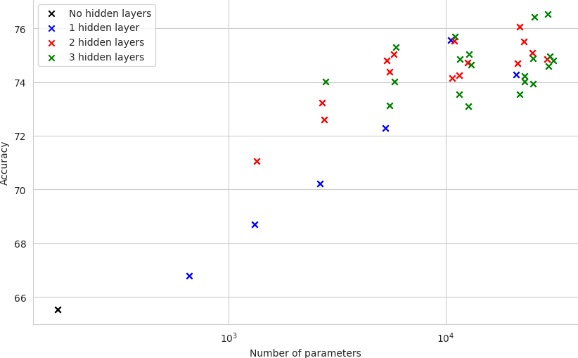
A few initial remarks can be made. The number of parameters is given in logarithmic scale for better visualization. The measurements are divided into three groups depending on the number of hidden layers of the underlying model: None (which corresponds to the simple perceptron model), one, two, and three hidden layers. As can be seen, the groups overlap (e.g., the model with one hidden layer of 128 neurons has more parameters than the model with two hidden layers of 8 and 4 neurons), but it is still possible to observe a separation between them.
At lower parameter counts, the accuracy of the model correlates with the number of neurons per layer. However, at some point, the increase in accuracy becomes marginal or even stagnates. As the model becomes more complex, the accuracy does not increase linearly with the number of neurons. Indeed, the model starts to memorize the training data instead of generalizing well to unseen data.
We now consider the question of how the proving costs increase with the number of neurons per layer. Since the proof-generation process is time consuming and we would like to have a statistically significant result (i.e., a few rounds), we run the bench_ezkl function on 50 rounds and report the average times with error margins.
The results are shown in the following plot, where the x-axis represents the number of parameters of the model and the y-axis represents the average time of the Setup, Prove, and Verify phases. In the last plot, we show the average value of logrows:
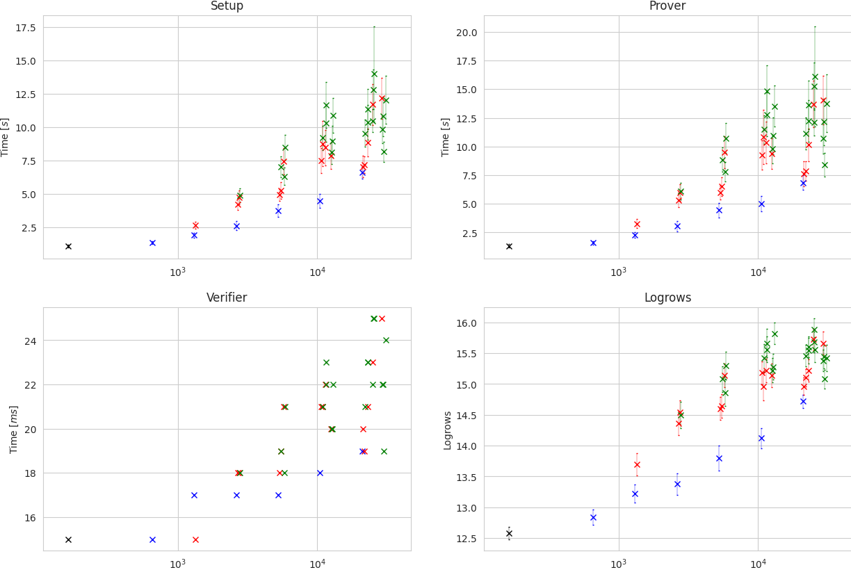
Comparing this plot to the previous one, one can observe that proving costs increase faster than model accuracy. If we consider only the models with one hidden layer (blue markers), the timings exhibit a clear linear growth (exponential-looking due to the logarithmic x-axis). However, once we introduce more hidden layers, time measurements are no longer exactly proportional to the number of parameters. This is indeed a general fact of circuit-based zkML: the proving time is not directly determined by the number of parameters of the model, but rather by the number of constraints in the arithmetic circuit, which is largely influenced by the model’s architecture. We explore this next.
Changing Model Architecture
In this final section, we compare the proving costs of different architectures. We consider the following Sklearn models: Support Vector Machines (SVMs) and Ridge Regression Classifiers. As previously mentioned, Sklearn models are not natively supported by EZKL, so we convert them to PyTorch models using the sk2torch library.
We select the best hyperparameters for each model using a grid search and evaluate the models on 50 rounds. We provide a brief overview of each model’s performance and the proving costs below:
Support Vector Machine (SVMs): SVMs are known for their ability to handle high-dimensional data and are particularly effective in cases where the number of features is greater than the number of samples. This is not the case in our dataset, since we have 162 features and 599 samples. However, in practice, SVMs can still yield good results when the number of features is in the same order of magnitude as the number of samples. Using a linear kernel and the default regularization parameter of 1, we obtain an accuracy of 0.73, which is slighly lower but comparable to the best models we have trained so far. In contrast, the proof costs are significantly lower, with average setup, prove, and verify times of 1.28, 1.72, and 0.014 seconds, respectively. The average value of
logrowsis 13.1.Ridge Classifier: Ridge regression is a linear regression model that uses L2 regularization to prevent overfitting. This is particularly useful when the dataset is noisy or when there are many features. We increase the regularization parameter to 10 and obtain an accuracy of 0.72, which is comparable to the SVM model. The proof costs are even lower, with average setup, prove, and verify times of 0.66, 0.84, and 0.013 seconds, respectively. The average value of
logrowsis 12.1. We can see that the Ridge Classifier is a good compromise between accuracy and proving costs and would be a good choice for a real-world application even if the accuracy is slightly lower than the best models.
Conclusion
In this article, we have explored various trade-offs in zkML. The experimental results illustrate the balance between model complexity, proving costs and prediction accuracy. Although these results are based on a simplified example and should be interpreted as a general guideline rather than a definitive conclusion, some key takeaways can be drawn from the analysis:
Increasing the complexity of the model can lead to linear growth in proving costs and yet diminishing returns for accuracy.
Proving costs are not exclusively determined by the number of parameters but also by the model’s architecture and the number of constraints in the arithmetic circuit.
In a nutshell, zkML should not be regarded as a one-size-fits-all solution. Instead of blindly porting a model into the zkML framework of choice, ML practitioners interested in verifiable inference should design their models with proving costs in mind from the beginning. Failing to do so and using frameworks such as EZKL or GIZA as a black box is likely to result in a suboptimal trade-off between proving costs and accuracy.
Author: César Descalzo